Sample Mean, Sample Variance, and Confidence Interval

If the internal components of a system behave stochastically or if its input events can occur at arbitrary times, the performance have randomness.

If we reset the model under study prior to each simulation run, the performance indices from each run are independent from those of all the other runs. Random variables are said to be identically distributed if the associated variables have identical measurement. For examples, the Utilization of Processor in BufferProcessor of Figure 4.1 from multiple simulation runs are independent and identically distributed (IID) random variable.

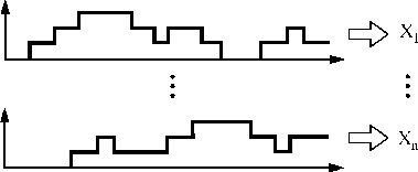
Figure 4.5: IID random variants $X_1 \ldots X_n$ from $n$ simulation runs

Suppose that we try to estimate the real mean $\mu$ of a random variable from a sample whose values are $X_1, X_2, \ldots X_n$ from $n$ simulation runs as illustrated in Figure 4.5. Then the sample mean

$$\hat{\mu}=\frac{\displaystyle{\sum_{i=1}^{n} X_i}}{n}$$ (5.8)

is an unbiased (point) estimator of the real mean $\mu$ . Similarly, the sample variance

$$\hat{\sigma}^2(n)=\frac{\displaystyle{\sum_{i=1}^{n} [X_i-\hat{\mu}]^2}}{n-1}$$ (5.9)

is an unbiased estimator of the real variance $\sigma^2$ . For $n \ge 2$ , a 100($1-\alpha$ ) percent confidence interval for $\mu$ is given by

$$\hat{\mu} \pm t_{n-1,1-\alpha/2}\sqrt{\frac{\hat{\sigma}^2(n)}{n}}$$ (5.10)

where $t_{n-1,1-\alpha/2}$ is the upper $1-\alpha/2$ critical point for the $t$ distribution with $n-1$ degree of freedom. It can be written

$$P\biggl[\hat{\mu}- t_{n-1,1-\alpha/2}\sqrt{\frac{\hat{\sigma}^2(n... ...hat{\mu}+ t_{n-1,1-\alpha/2}\sqrt{\frac{\hat{\sigma}^2(n)}{n}} \biggr]=1-\alpha$$ (5.11)

and we say that we are 100(1-$a$ ) percent confident that the real $\mu$ lies in the interval given by Equation (4.10).

Example 5.5   Suppose that 10 simulation runs produce system throughput data of 12.0, 15.0, 16.8, 18.9, 9.5, 14.9, 15.8, 15.5, 5.0, and 10.9. Our objective is to build the 90 % confidence interval for $\mu$ . We have t-distribution values of $t_{10,0.9}$ =1.372, $t_{10,0.95}$ =1.812, $t_{9,0.9}$ =1.383, $t_{9,0.95}$ =1.833.

Then $\hat{\mu}$ =13.4 and $\hat{\sigma}^2$ =1.7 and the 90% confidence interval for $\mu$ is $\hat{\mu}\pm t_{9,0.95}\sqrt{\frac{\hat{\sigma}^2(n)}{n}}=13.4\pm1.83\sqrt{\frac{1.7}{10}}=13.4\pm0.75$ $\square$

The values of $t_{n-1,1-\alpha/2}$ of $t$ pdf are available in many statistics books and simulation books [Zei76,LK91]. DEVS++ calculates the 100(1-$\alpha$ ) confidence interval for $\mu$ when using mrun n for $2 \le$ n$\le 20$ in verion 1.4.1We will see it in detail in Section 4.3.